Asset Allocation Basics
The Cornerstone of Portfolio Construction and Risk Management
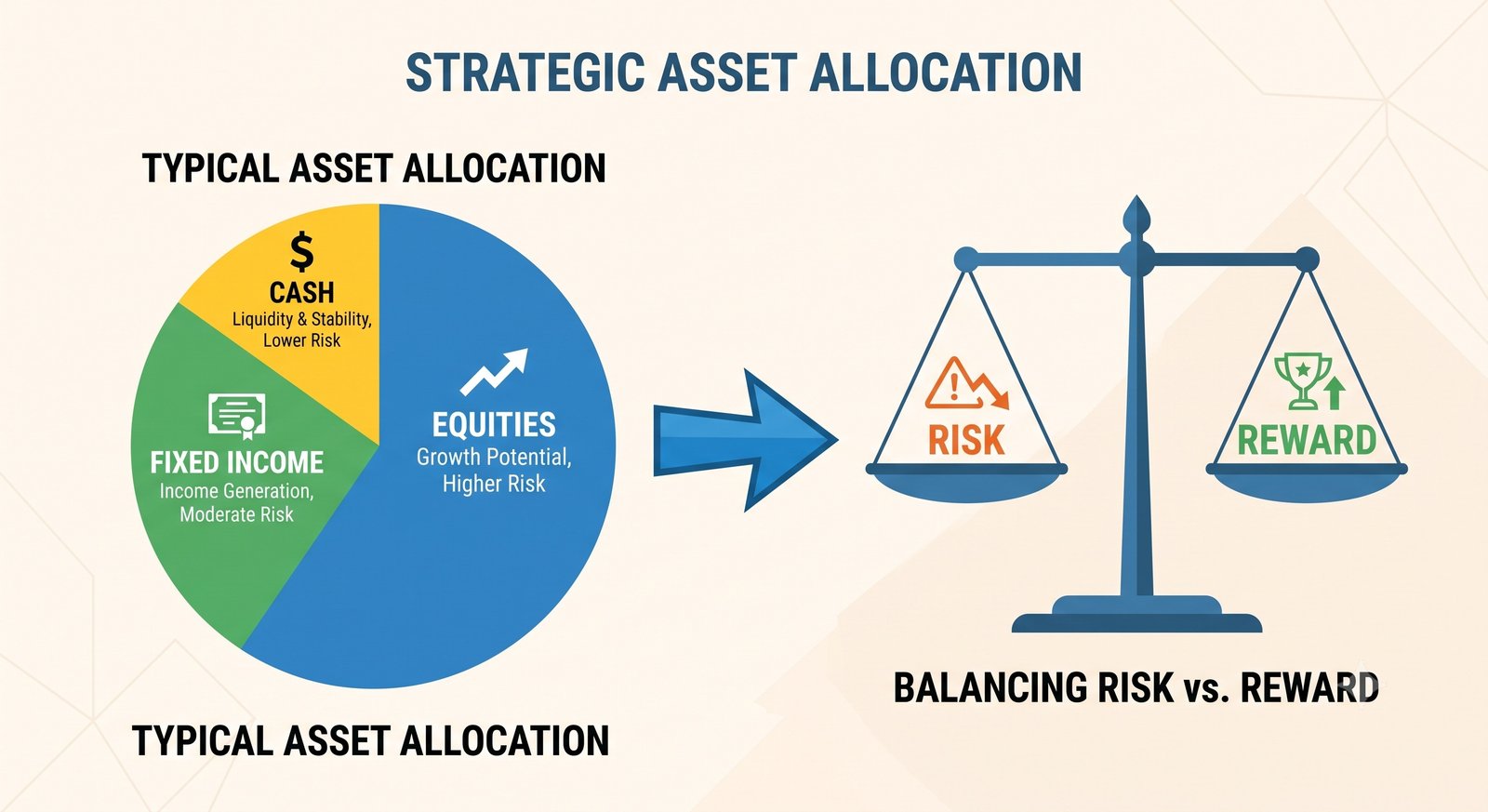
Asset allocation is the fundamental investment strategy of dividing an investment portfolio across various asset class categories, such as equities, fixed income, cash equivalents, and alternative investments. This division is heavily dictated by an investor's specific time horizon, risk tolerance, and overarching financial goals. Unlike individual stock selection or market timing—which attempt to generate excess returns through prediction and active management—asset allocation operates on the macroeconomic principle of diversification. The central thesis is that different asset classes exhibit varying degrees of correlation with one another; they rarely move in perfect tandem under the same economic conditions. By combining non-correlated or negatively correlated assets, investors can optimize the risk-to-reward ratio of their portfolios.
Extensive empirical research in financial economics, most notably the landmark 1986 study by Gary Brinson, L. Randolph Hood, and Gilbert Beebower, demonstrated that asset allocation policy dictates over 90% of the variance in portfolio returns over time, deeply overshadowing individual security selection and market timing. Therefore, mastering the basics of asset allocation is not merely an optional enhancement for an investor, but the structural foundation upon which all enduring wealth accumulation and preservation strategies are built.
1. Theoretical Foundations: Modern Portfolio Theory (MPT)
The intellectual bedrock of asset allocation was established by Harry Markowitz in 1952 with the introduction of Modern Portfolio Theory (MPT), a contribution that later earned him the Nobel Memorial Prize in Economic Sciences. MPT mathematically formalized the concept of diversification. Prior to Markowitz, investors largely focused on identifying individual securities that offered the highest potential return. Markowitz shifted the paradigm by proving that the risk of an individual asset should not be evaluated in isolation, but rather by how its price movement impacts the overall volatility of a combined portfolio.
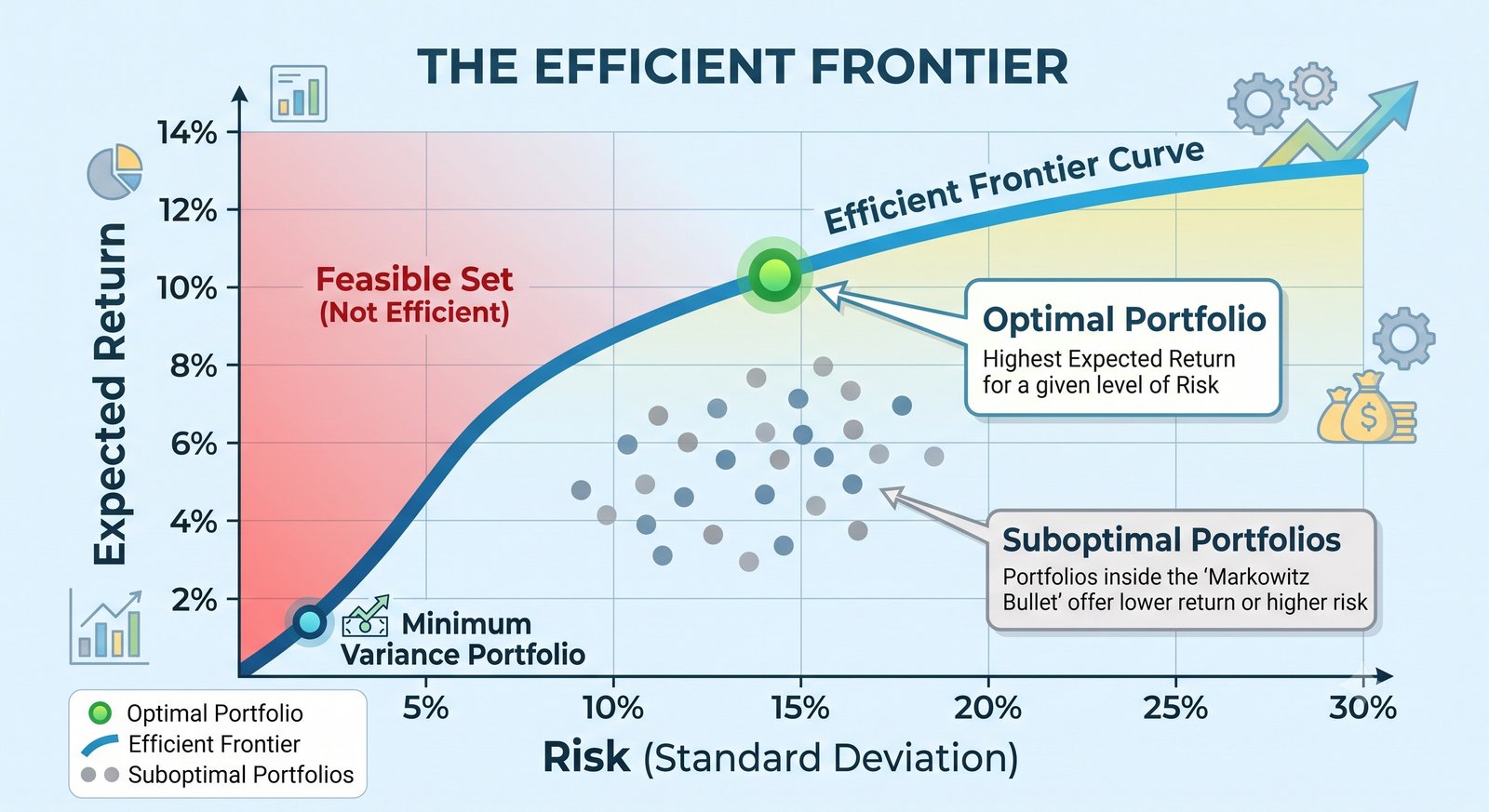
The primary mechanism of MPT relies on the statistical measure of covariance and correlation between different assets. If Asset A declines during a specific economic shock (e.g., a rapid increase in interest rates), but Asset B rises or remains stable during that same shock, holding both assets simultaneously reduces the portfolio's aggregate volatility without necessarily sacrificing proportional return. This phenomenon gives rise to the Efficient Frontier, a theoretical curve representing a set of optimal portfolios that offer the highest expected return for a defined level of risk.
- Idiosyncratic Risk (Unsystematic): Risk inherent to a specific company or sector (e.g., a CEO scandal or a localized supply chain disruption). Asset allocation and diversification effectively eliminate this risk.
- Systematic Risk (Market Risk): The macroeconomic risks that affect the entire market (e.g., global recessions, inflation, wars). While systematic risk cannot be entirely diversified away, cross-asset allocation (e.g., holding gold or sovereign debt alongside equities) mitigates its impact.
- The Efficient Frontier: Portfolios that lie on this curve are considered optimized. Any portfolio falling below the curve is sub-optimal because a mathematically superior allocation exists that could provide higher returns for the identical risk level.
2. Deep-Dive Explanations & Formulas: The Mathematics of Allocation
To truly understand asset allocation, one must look beneath the conceptual framework and examine the driving mathematics. The expected performance of a portfolio is calculated using weighted averages, while the risk (measured by variance or standard deviation) requires a more complex calculation involving the correlation coefficient ($\rho$) between the respective assets.
Expected Return of a Portfolio: The expected return is simply the proportional sum of the expected returns of the individual assets within the portfolio.
$$E(R_p) = \sum_{i=1}^{n} w_i E(R_i)$$
Where $E(R_p)$ is the expected portfolio return, $w_i$ is the percentage weight of asset $i$ in the portfolio, and $E(R_i)$ is the expected return of asset $i$.
Portfolio Variance (Risk): The formula for the risk of a two-asset portfolio highlights the magic of diversification. It incorporates the standard deviation ($\sigma$) of each asset, their weights, and crucially, their correlation coefficient ($\rho_{1,2}$).
$$\sigma_p^2 = w_1^2 \sigma_1^2 + w_2^2 \sigma_2^2 + 2w_1w_2\sigma_1\sigma_2\rho_{1,2}$$
Because the correlation coefficient ($\rho_{1,2}$) scales from -1.0 (perfectly negatively correlated) to +1.0 (perfectly positively correlated), adding an asset with a correlation of less than 1.0 will geometrically reduce the total variance $\sigma_p^2$. If the correlation is 0 or negative, the third term in the equation shrinks or subtracts from total risk, thereby protecting the investor during drawdowns.
The Sharpe Ratio: To measure how well a specific asset allocation is performing relative to the risk it assumes, modern finance utilizes the Sharpe Ratio. It calculates the excess return generated per unit of standard deviation.
$$S = \frac{R_p - R_f}{\sigma_p}$$
Where $R_p$ is portfolio return, $R_f$ is the risk-free rate (like sovereign Treasury yields), and $\sigma_p$ is the portfolio's standard deviation. Efficient asset allocation strategies aim to maximize this ratio, ensuring that the investor is adequately compensated for the volatility they endure.
3. Core Asset Classes & Macroeconomic Mechanics
Successful allocation requires a deep understanding of how different asset classes react to distinct macroeconomic environments—primarily the phases of economic growth (expansion vs. recession) and monetary environments (inflation vs. deflation).
- Equities (Stocks): Represent ownership in corporations. They are the primary engine for long-term growth and capital appreciation. Historically, equities outpace inflation over long horizons. Mechanically, equity valuations are sensitive to corporate earnings and prevailing interest rates. They perform best in low-inflation, high-growth environments but suffer severe drawdowns during liquidity crises and recessions.
- Fixed Income (Bonds / Debt Instruments): Represent loans made by the investor to a borrower (corporate or government). They provide regular interest income and capital preservation. Bond prices share an inverse mechanical relationship with interest rates: as central banks raise rates to fight inflation, existing bond prices fall. However, high-grade sovereign bonds generally act as a deflationary hedge, spiking in value when equities crash as investors flee to safety.
- Cash and Equivalents: Includes highly liquid instruments like liquid mutual funds, Treasury bills, or money market accounts. Cash provides ultimate safety of principal and immediate liquidity, offering optionality to deploy capital during market corrections. However, cash is uniquely vulnerable to inflation, which erodes its real purchasing power over time.
- Alternatives (Gold, Real Estate, Commodities): These assets behave differently than traditional stocks and bonds. Gold, for instance, has historically served as a non-yielding monetary asset that performs well during periods of systemic mistrust, currency debasement, or stagflation. Real estate offers physical utility, rental yield, and acts as a natural inflation hedge since property values and rents generally rise alongside consumer prices.
4. Structured Comparison: Analyzing Asset Class Attributes
Understanding the granular differences in risk, return, and utility is critical for building a target allocation. The table below illustrates the generalized profiles of these core asset categories.
| Asset Class | Historical Volatility (Risk) | Primary Economic Function & Inflation Protection |
|---|---|---|
| Equities (Large Cap) | High | Capital appreciation; Strong long-term inflation hedge via corporate pricing power. |
| Fixed Income (Govt Bonds) | Low to Moderate | Capital preservation & income; Poor inflation hedge but excellent deflationary hedge. |
| Cash & Liquid Equivalents | Zero to Negligible | Absolute liquidity & safety of principal; Negative real returns during inflationary periods. |
| Gold / Precious Metals | Moderate to High | Store of value; Strong hedge against currency debasement and geopolitical tail risks. |
5. Strategic vs. Tactical Asset Allocation
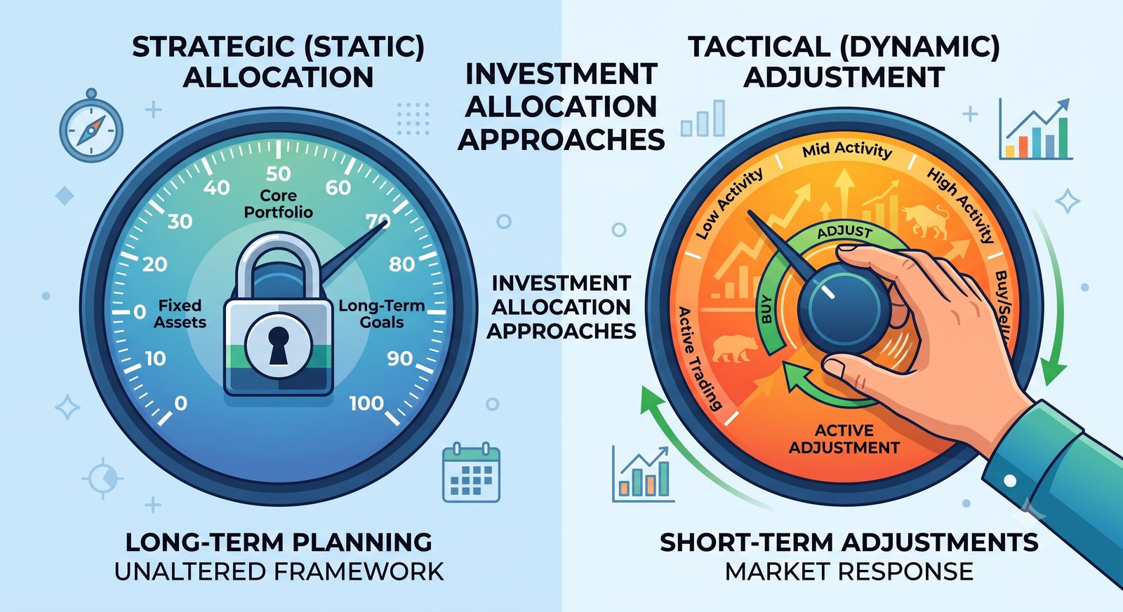
Asset allocation models generally fall into two distinct philosophical camps: Strategic and Tactical.
Strategic Asset Allocation (SAA): This is a "buy-and-hold" methodology tied directly to the investor's baseline goals. An investor defines a base policy mix (e.g., 60% equities, 40% bonds) based on long-term capital market expectations and personal risk tolerance. The only action taken in SAA is periodic rebalancing. When market movements cause the actual portfolio weights to drift significantly from the target (e.g., a bull market pushes equities to 75%), the investor mechanical sells the outperforming asset and buys the underperforming asset to return to the 60/40 target. This imposes a strict discipline of buying low and selling high, mitigating emotional bias.
Tactical Asset Allocation (TAA): Tactical allocation is a more active approach that permits short-term deviations from the strategic mix to capitalize on unusual or exceptional market opportunities. For example, if a tactical investor’s baseline strategy is 60/40, but leading economic indicators forecast a severe, imminent recession, they might tactically shift to 40% equities and 60% bonds. Once the economic storm passes, they revert to their strategic baseline. While TAA offers the potential to enhance risk-adjusted returns, it introduces timing risk and requires significant macroeconomic expertise to execute successfully without eroding wealth through mistimed trades and transaction costs.
6. Realistic Case Studies
To contextualize the theoretical frameworks of asset allocation, we examine two practical, edge-case scenarios demonstrating how different allocations function mathematically and behaviorally across distinct life stages.
- Case Study 1: The Accumulator (Growth & Volatility Harvesting)
Profile: Sarah, 32 years old, highly stable income as an aerospace engineer. Goal: Retirement in 30 years.
Allocation: 85% Equities (broad domestic & international indices) / 15% Fixed Income (medium-duration bonds).
Scenario in Action: A sudden global black swan event causes the equity market to drop by 40% over three months. Sarah's portfolio mathematically drifts from 85/15 to approximately 70% Equities and 30% Bonds. Because her time horizon is three decades, her risk capacity is exceptionally high. Following her Strategic Asset Allocation rules, she executes an annual rebalance. She sells off a portion of her bonds (which held their value or increased due to a flight-to-safety) and uses the proceeds to buy discounted equities to restore the 85/15 split. By doing this mechanically, she harvests the volatility. When the equity market eventually recovers, she holds significantly more equity shares than she did prior to the crash, accelerating her compound growth trajectory. - Case Study 2: The Retiree (Capital Preservation & Sequence Risk)
Profile: David, 65, recently retired. Relies on a Systematic Withdrawal Plan (SWP) to fund his lifestyle. Goal: Generate income and prevent capital depletion over a 25-year horizon.
Allocation: 40% Equities / 50% Fixed Income & Debt Funds / 10% Cash Equivalents & Gold.
Scenario in Action: David faces "Sequence of Returns Risk"—the danger of experiencing severe market declines early in retirement while actively withdrawing funds, permanently crippling the portfolio's longevity. A protracted bear market hits during year two of his retirement, slashing equity values. If David were 100% in equities, withdrawing funds would force him to sell shares at rock-bottom prices, locking in irreversible losses. However, because of his 40/50/10 allocation, he leaves the battered equities untouched to allow them time to recover. He instead funds his living expenses by withdrawing from the 10% Cash and liquidating portions of his 50% Fixed Income sleeve. This strategic buffer insulates his core equity growth engine, ensuring his portfolio survives the bear market without structural damage.
7. Actionable Strategy Guide: Step-by-Step Implementation
Implementing an optimal asset allocation strategy is a systematic process. By following these rigorous steps, an investor can transition from theoretical understanding to practical application.
- Step 1: Quantify Time Horizon and Objective. The most dominant variable is time. Money required within 0-3 years (like a home down payment) belongs almost entirely in cash equivalents or short-term debt, neutralizing market volatility. Wealth aimed at goals 10+ years away should heavily overweight equities to combat long-term inflation.
- Step 2: Differentiate Between Risk Tolerance and Risk Capacity. Tolerance is psychological: how well you sleep at night during a 20% portfolio drop. Capacity is mathematical: how much financial loss you can withstand without altering your lifestyle. Your allocation must be anchored to the lower of these two metrics. An investor with high capacity but low tolerance will panic-sell if allocated too aggressively, destroying their compounding efforts.
- Step 3: Define Your Target Allocation (The Policy Portfolio). Select a precise model tailored to your findings in Steps 1 and 2. Common baseline templates include Conservative (20% Equity/80% Fixed Income), Balanced (60% Equity/40% Fixed Income), and Aggressive Growth (80%-100% Equity). Write this down in an Investment Policy Statement (IPS) to serve as an emotional anchor during market turbulence.
- Step 4: Select the Underlying Instruments. Populate your broad asset classes with highly efficient, low-cost vehicles. Instead of attempting to pick winning individual stocks, utilize broad-market index funds or Exchange-Traded Funds (ETFs) to capture the pure asset class return (beta) without idiosyncratic risk.
- Step 5: Establish a Mechanical Rebalancing Protocol. Choose a rebalancing trigger to avoid portfolio drift. This can be time-based (e.g., executing a rebalance on the first trading day of January every year) or tolerance-band based (e.g., rebalancing only when an asset class drifts by 5% or more from its target weight). Automating this process removes subjective human emotion from the equation.
Frequently Asked Questions
Q: How frequently should I rebalance my asset allocation?
Research indicates that excessively frequent rebalancing (e.g., monthly) can lead to a drag on returns due to transaction costs and tax friction, without significantly reducing volatility. A widely accepted best practice is to rebalance annually, or to utilize a "tolerance band" approach—rebalancing only when an asset class deviates from its target allocation by an absolute 5 to 10 percentage points. Additionally, directing new capital contributions to underweight asset classes can effectively rebalance a portfolio without incurring taxable events.
Q: Does proper asset allocation guarantee that I won't lose money?
No. Asset allocation does not eliminate risk; it manages and optimizes it. Systematic risk—the possibility of an entire market collapsing due to macroeconomic shocks—will still cause a diversified portfolio to lose value in the short term. However, effective asset allocation ensures that the decline is mathematically dampened by non-correlated assets, minimizing drawdown severity and significantly improving the speed of recovery compared to an un-diversified portfolio.
Q: Is a traditional 60/40 portfolio (60% Equities, 40% Bonds) still effective today?
The 60/40 portfolio is a classic benchmark that provides a robust balance of growth and capital preservation. However, its effectiveness has been scrutinized during periods of simultaneous stock and bond market declines—typically triggered by sudden, massive inflation shocks causing central banks to rapidly raise interest rates. To fortify the 60/40 model in highly inflationary environments, many institutional investors now integrate a 10% to 15% alternative sleeve (gold, commodities, real estate) creating variations like a 50/35/15 model to ensure protection across all monetary conditions.
Q: How does age factor into my asset allocation decision?
Age is typically a proxy for investment time horizon and human capital. A popular rule of thumb is "100 minus your age" (or "120 minus your age" for longer life expectancies) to determine your equity allocation. A 30-year-old might hold 90% in equities due to their ability to endure multiple boom-and-bust cycles while earning a salary. A 70-year-old has less time to recover from a severe market crash and a heavier reliance on portfolio income, necessitating a much larger allocation to stable, fixed-income assets to mitigate sequence of returns risk.
See also
- Loading related topics...