Compound Interest Mechanics
The Definitive Guide to Exponential Capital Growth, Yield Geometry, and Financial Temporal Dynamics
In the advanced study of macroeconomics, institutional wealth management, and quantitative finance, compound interest is unequivocally the foundational mathematical principle driving all long-term capital accumulation, debt amortization, and asset valuation models. Unlike simple interest—an elementary and linear financial mechanic which calculates yield exclusively and perpetually on the original principal amount deposited—compound interest introduces a recursive, dynamic variable: it calculates yield on both the original principal and the accumulated interest from all preceding periods. This fundamental structural divergence shifts the trajectory of capital growth from a flat, predictable linear arithmetic progression to an aggressive, compounding geometric exponential curve.
Often apocryphally attributed to theoretical physicist Albert Einstein as the "eighth wonder of the world," compounding is the explicit mathematical engine that allows modest, systematic retail savings to evolve into immense, multi-generational institutional wealth over extended temporal horizons. The operational reality of compound interest essentially mandates that fiat currency transcends its role as a static medium of exchange and transforms into an autonomous, self-replicating entity. If a depositor earns a specific yield in year one, that newly generated interest immediately becomes part of the principal base for year two. Consequently, year two will inherently generate a larger absolute monetary return than year one, even if the benchmark macroeconomic interest rate remains entirely static. This recursive, self-reinforcing cycle accelerates profoundly over time, creating a "snowball effect" that mathematically dominates and ultimately neutralizes short-term market volatility.
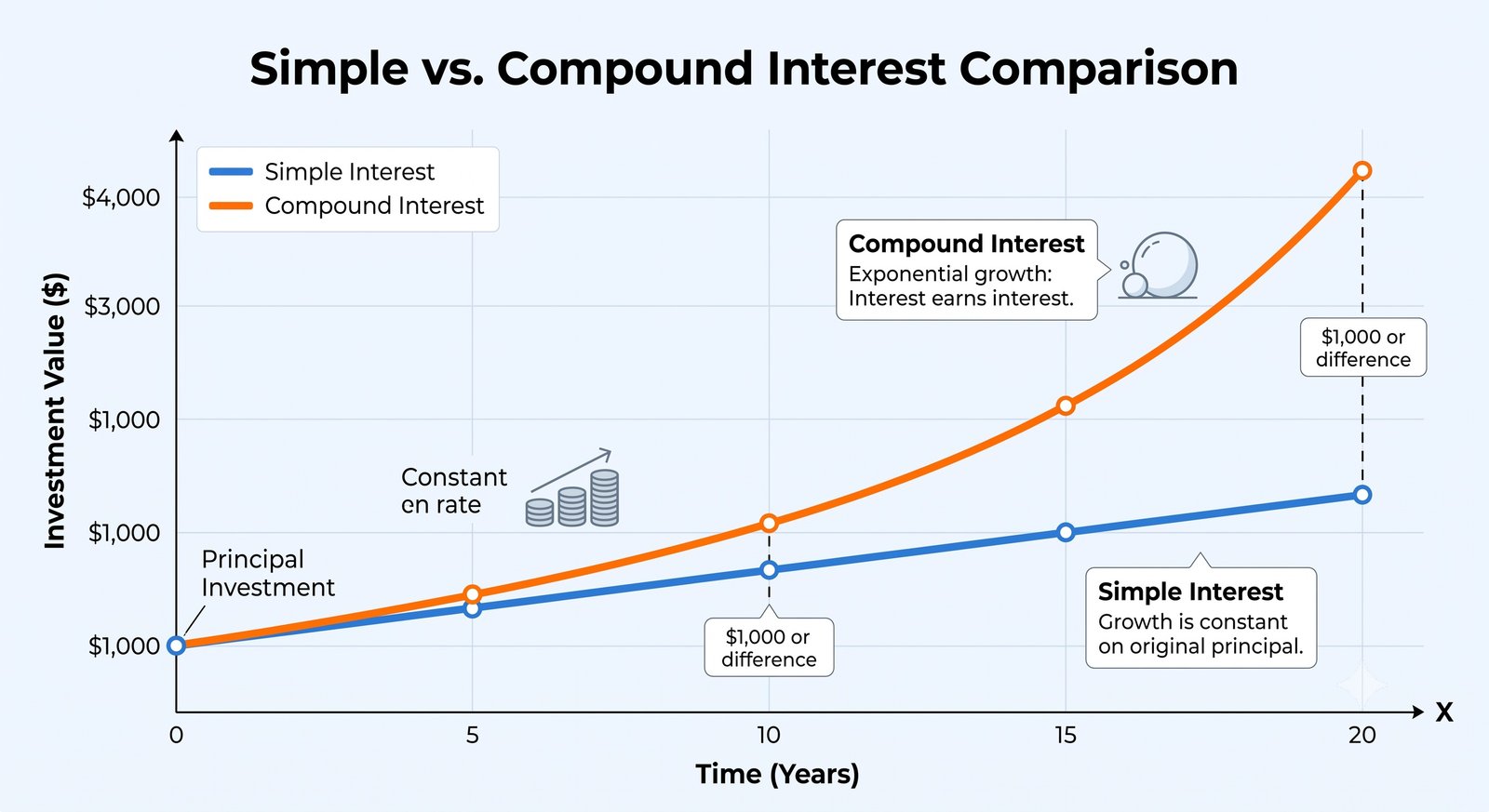
However, the exact same mathematical properties that systematically build massive wealth for disciplined investors also act as a devastating, predatory financial mechanism against uneducated borrowers. When applied to revolving credit facilities, residential mortgages, and uncollateralized consumer debt, compound interest rapidly accelerates the total liability owed. It frequently traps mathematically illiterate consumers in perpetual, inescapable debt cycles where their minimum periodic payments fail to cover the newly compounded interest, resulting in negative amortization. Therefore, mastering the intricate calculus of compounding, understanding the massive impact of compounding frequency, and respecting the critical importance of temporal duration is the absolute, non-negotiable prerequisite for fiduciary-level financial sovereignty.
1. The Deep-Dive: Mathematical Foundation and Core Formulas
The precise calculation of exponential capital growth is governed by the standard compound interest formula utilized by banking actuaries, derivative pricing models, and financial institutions globally. To successfully operationalize and project wealth using this equation, an investor must intimately understand its constituent variables, as manipulating any single input drastically and non-linearly alters the ultimate financial trajectory of the asset.
The Universal Compound Interest Formula:
A = P × (1 + r/n)^(n × t)
- A (Total Amount / Future Value): The final future value of the investment or loan, encompassing both the initial principal injection and all accumulated, compounded interest over the total lifespan of the asset.
- P (Principal): The initial lump sum of capital deposited, invested, or borrowed at the absolute inception of the financial contract.
- r (Annual Nominal Interest Rate): The stated annual interest rate, unconditionally expressed as a decimal within the formula (e.g., an 8.5% yield is rendered as 0.085).
- n (Compounding Frequency): The total number of discrete times the interest is calculated and added back to the principal balance per single calendar year (e.g., 1 for annually, 4 for quarterly, 12 for monthly, 365 for daily).
- t (Time/Temporal Duration): The total lifespan of the investment or loan, uniformly expressed in years. Because it operates as an exponent in the equation, 't' is the most mathematically powerful variable in the formula.
Continuous Compounding (The Theoretical Limit): In advanced institutional finance and options pricing (such as the Black-Scholes model), analysts frequently utilize continuous compounding. This theoretical framework assumes interest is calculated and added to the principal at every infinitesimally small fraction of a microsecond. The formula introduces Euler's number (e, approximately 2.71828) as the mathematical limit: A = P × e^(rt). While retail bank accounts do not compound continuously, understanding this limit demonstrates the absolute maximum theoretical yield an interest rate can generate.
2. Compounding Frequency: The Dichotomy of APY versus APR
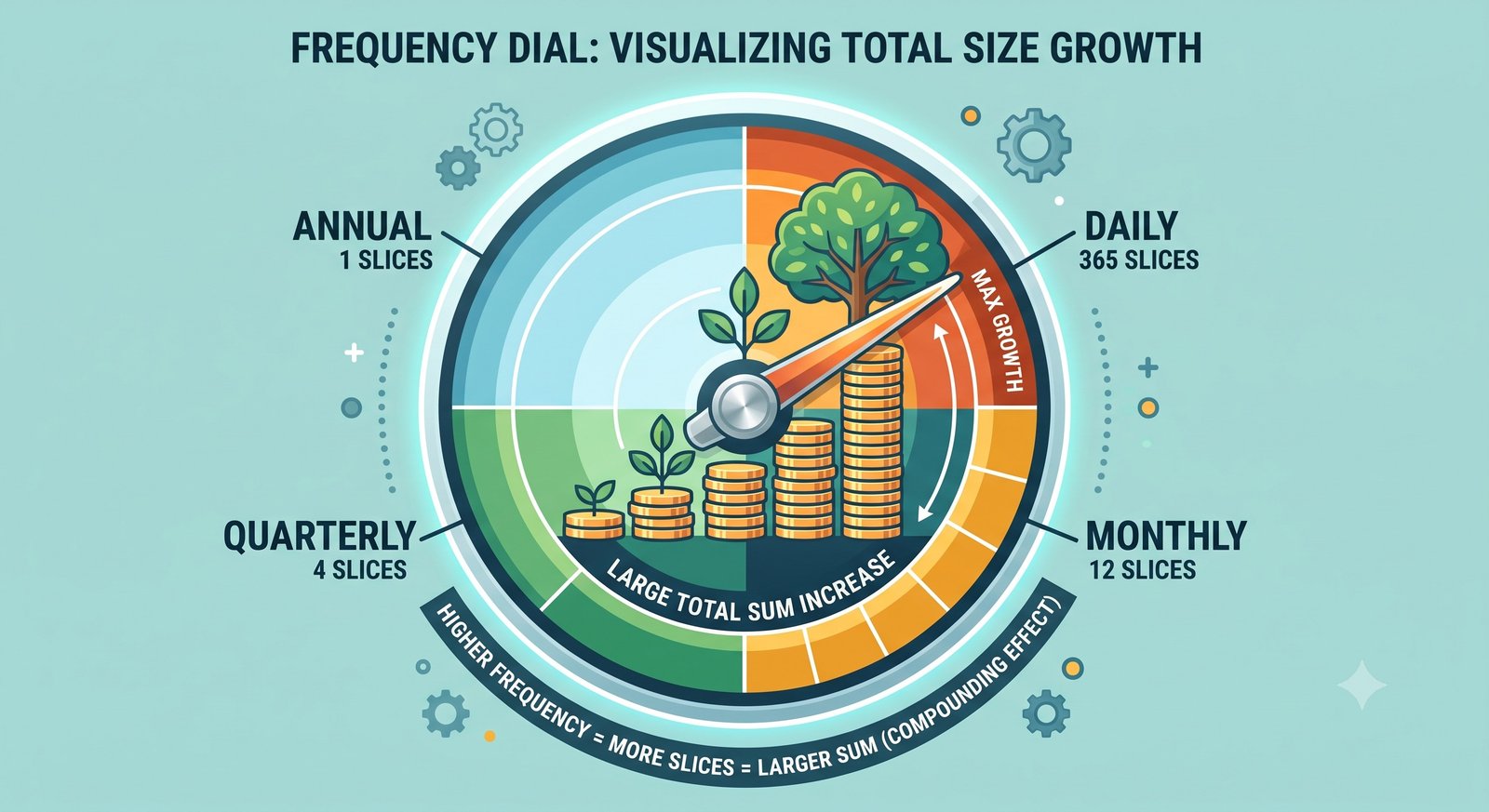
The frequency at which interest is compounded (the 'n' variable) is a critical, often weaponized lever in financial engineering. Interest does not have to be applied exclusively at the end of a 365-day calendar year; depending on the institutional contract, it can be compounded semi-annually, quarterly, monthly, or daily. The fundamental mathematical axiom is resolute: the higher the compounding frequency, the greater the final exponential growth. This occurs because the newly generated interest begins generating its own subsequent returns much sooner in the operational cycle.
This mechanical reality creates a critical, legally mandated distinction between two standard retail banking terms: Annual Percentage Rate (APR) and Annual Percentage Yield (APY). APR represents the simple, nominal interest rate stated on the financial product without factoring in the mathematical effect of intra-year compounding. Conversely, APY—also known in corporate finance as the Effective Annual Rate (EAR)—calculates the true, precise mathematical yield by explicitly factoring in the compounding frequency.
Effective Annual Yield (APY) Formula:
APY = (1 + r/n)^n - 1
For instance, a credit card carrying a nominal 24% APR that compounds daily (n=365) will actually subject the borrower to an Effective Annual Yield (APY) of approximately 27.11%. Regulatory frameworks (such as the Truth in Savings Act in the US) typically mandate that retail banks heavily advertise the higher APY metric for consumer deposit accounts to make savings products appear more lucrative, while concurrently advertising the lower nominal APR metric for consumer debt products to make borrowing appear falsely inexpensive. Recognizing this institutional asymmetry is critical for evaluating true financial costs.
3. Structural Comparison: The Impact of Compounding Frequency
To visualize the profound impact of compounding frequency over extended temporal horizons, we evaluate a static $100,000 principal investment generating a constant 8.00% nominal return. As demonstrated below, while the difference between frequencies appears negligible in Year 1, the mathematical divergence becomes staggering by Year 30 due to the exponential expansion of the principal base.
| Compounding Frequency (n) | Future Value (Year 10) | Future Value (Year 20) | Future Value (Year 30) |
|---|---|---|---|
| Simple Interest (No Compounding) | $180,000.00 | $260,000.00 | $340,000.00 |
| Annually (n=1) | $215,892.50 | $466,095.71 | $1,006,265.69 |
| Quarterly (n=4) | $220,803.97 | $487,543.92 | $1,076,516.30 |
| Monthly (n=12) | $221,964.02 | $492,680.28 | $1,093,572.97 |
| Daily (n=365) | $222,534.58 | $495,216.40 | $1,102,027.76 |
Analysis: The table demonstrates that moving from an annual compounding schedule to a daily compounding schedule yields nearly $100,000 in additional free capital over a 30-year horizon, assuming the exact same principal and nominal interest rate. It also highlights the catastrophic mathematical failure of simple interest, which trails daily compounding by over three-quarters of a million dollars in Year 30.
4. Empirical Case Studies: The Temporal Vector
While securing a high nominal interest rate is highly beneficial, the single most dominant and unforgiving variable in the compound interest formula is time ('t'). Because time serves as the exponential power in the algebraic equation, the duration capital remains invested exerts a vastly disproportionate, non-linear impact on final wealth generation compared to the absolute principal amount injected.
Case Study 1: The Early Saver vs. The Late Sprinter (The Opportunity Cost of Delay)
Scenario: Consider two hypothetical investors, Eleanor and Julian, both targeting retirement at age 65. They both invest in an identical S&P 500 ETF generating a historical annualized return of 8%, compounded monthly.
• Eleanor (The Early Saver): Begins investing $500 monthly at age 25. She does this for exactly 10 years until age 35, contributing a total out-of-pocket principal of $60,000. At age 35, she completely stops contributing, but leaves the accumulated capital untouched to compound for the next 30 years until age 65.
• Julian (The Late Sprinter): Delays investing entirely during his twenties. At age 35, realizing he is behind, he begins investing $500 monthly. He does this relentlessly, every single month for 30 years until age 65, contributing a total out-of-pocket principal of $180,000.
The Mathematical Resolution:
Eleanor's 10 years of initial contributions grow to $91,473 by age 35. That lump sum then sits untouched, compounding at 8% for 30 more years. Her final balance at age 65 is $999,996.00.
Julian's 30 years of continuous, grueling $500 monthly payments compound concurrently. His final balance at age 65 is $745,179.00.
Analysis: Despite Julian investing three times more physical fiat capital out of his own pocket ($180,000 vs $60,000) and sacrificing his cash flow for three decades, Eleanor retires with over a quarter-million dollars more in total wealth. The extra decade of unmolested compounding time allowed Eleanor's early capital to achieve an exponential "breakaway velocity" that Julian's later, heavier capital injections could mathematically never catch.
Case Study 2: The Wealth-Destroying Power of Compound Debt
Scenario: Marcus (28) carries an $8,000 balance on a premium rewards credit card following a vacation. The credit card issuer charges an APR of 22.5%, which is calculated and compounded daily. To preserve his monthly cash flow, Marcus decides he will only pay the required "Minimum Payment" each month, which the bank calculates as 2% of the outstanding balance, or $160.
The Mathematical Resolution: In month one, the 22.5% daily compounded APR generates approximately $150 in new interest. When Marcus pays his $160 minimum payment, $150 goes entirely to the bank as pure profit, and only $10 is applied to reduce the $8,000 principal. In month two, interest compounds on $7,990. If Marcus continues to only pay the minimum, it will take him roughly 112 months (over 9 years) to eradicate the debt. More devastatingly, over that 9-year horizon, Marcus will pay the bank over $9,800 in pure interest.
Analysis: Marcus effectively paid nearly $18,000 for an $8,000 vacation. The credit card issuer weaponized the daily compounding frequency against the borrower, mathematically ensuring that the asset (the loan) generated an exponential return for the bank's shareholders while financially paralyzing the consumer.
5. Advanced Heuristics: The Rule of 72, 114, and 144
Because complex exponential mathematics with fractional exponents are extremely difficult to calculate without institutional digital modeling tools, financial professionals, venture capitalists, and traders frequently employ robust mathematical heuristics to rapidly estimate compounding timelines. The most famous is the Rule of 72, accompanied by its corollaries, the Rule of 114 and the Rule of 144.
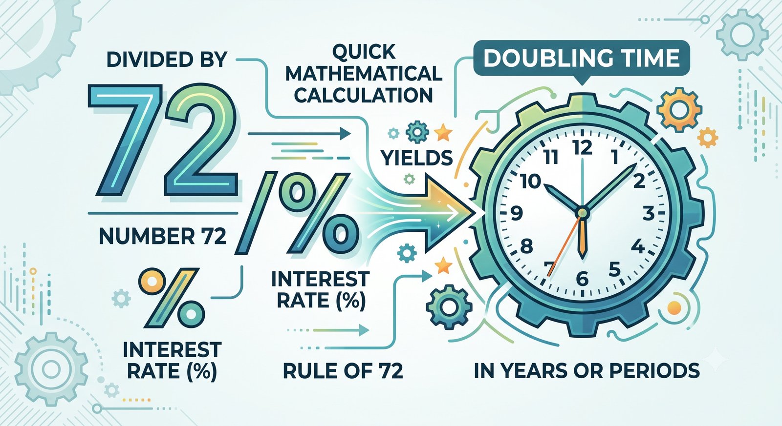
- The Rule of 72 (Doubling Time): This heuristic allows an investor to rapidly estimate the exact number of years required for an investment principal to double in value at a fixed annual rate of compound interest. You simply divide the integer 72 by the expected annual interest rate. If an S&P 500 index fund returns 8% annually, dividing 72 by 8 yields 9. It will take approximately 9 years for the invested capital to mathematically double.
- The Rule of 114 (Tripling Time): Utilized for longer-term planning, this formula dictates how long capital takes to triple. Divide 114 by the interest rate. At an 8% return, 114 / 8 = 14.25. The initial capital will triple in just over 14 years.
- The Rule of 144 (Quadrupling Time): To calculate when capital will multiply by four (quadruple), divide 144 by the interest rate. At an 8% return, 144 / 8 = 18. The portfolio quadruples every 18 years.
While they are heuristic approximations derived from natural logarithms rather than absolute precise algebraic metrics, these rules are highly accurate for interest rates falling between 5% and 12%. They serve as invaluable mental models for rapidly evaluating the long-term viability of investment prospects, negotiating corporate financing, and visually conceptualizing the compounding curve.
6. Actionable Strategy Guide: Engineering an Exponential Portfolio
Understanding the theory of compounding is useless without rigid operational execution. To weaponize compound interest for your own balance sheet and prevent institutional lenders from using it against you, implement the following step-by-step financial architecture:
- Step 1: Terminate All Daily Compounding Liabilities. Immediate triage is required if you carry unsecured credit card debt. Because credit card interest compounds daily at massive APRs, it is mathematically impossible to out-invest it. Liquidate low-yield savings, halt all non-matched retirement contributions, and aggressively deploy 100% of surplus cash flow to eradicate revolving debt. Alternatively, execute a balance transfer to a 0% APR promotional card to temporarily halt the compounding mechanism while paying down the principal.
- Step 2: Optimize the "n" Variable for Cash Equivalents. Review your emergency fund and liquid cash reserves. Move all fiat currency from legacy banks (compounding annually or monthly at 0.01%) to High-Yield Savings Accounts (HYSAs) that compound daily and pay out monthly. While the APY is the key metric, daily compounding ensures every dollar deposited immediately begins working the next morning.
- Step 3: Front-Load Investment Capital. Acknowledge the absolute supremacy of the 't' (time) variable. If you receive a financial windfall (tax refund, corporate bonus, inheritance), do not dollar-cost average it over two years. Execute a lump-sum investment immediately. Moving capital into the compounding curve earlier permanently expands the principal base for all future exponential calculations.
- Step 4: Automate the Reinvestment Loop (DRIPs). If you invest in dividend-paying equities or mutual funds, you must explicitly enable a Dividend Reinvestment Plan (DRIP) with your brokerage. If dividends are paid out as cash to your checking account, you break the compounding cycle. A DRIP automatically uses generated dividends to purchase fractional shares of the underlying asset, forcefully expanding the principal base without requiring new out-of-pocket capital.
- Step 5: Never Interrupt Unnecessary Compounding. Avoid liquidating long-term equity portfolios to fund short-term liabilities (like purchasing a vehicle) if low-interest financing is available. Selling $40,000 of an index fund resets the exponential curve for that specific capital block back to zero, destroying decades of future compounding potential to save a few hundred dollars in short-term auto loan interest.
7. Frequently Asked Questions (FAQ)
Q: Does compound interest still work if the stock market goes down during a recession?
Yes, but the mechanism alters. In a guaranteed fixed-income account (like a CD or Savings Account), compounding is mathematically continuous and linear; the balance never drops. In the equity markets (stocks/index funds), compounding is not a perfectly smooth curve because returns are highly volatile. You might gain 20% one year, lose 15% the next, and gain 10% the third. This is why financial planners use the Compound Annual Growth Rate (CAGR) to measure the smoothed, annualized return over a long horizon. As long as the long-term CAGR remains positive and you reinvest all dividends, the portfolio will recover from recessions and achieve the exponential trajectory calculated by the compounding formula.
Q: If compounding is so powerful, why do banks offer Simple Interest loans?
Banks generally do not offer simple interest loans. The vast majority of consumer auto loans and residential mortgages utilize heavily amortized compound interest. While they may be colloquially referred to as "simple interest" because the interest is calculated based on the daily remaining principal balance rather than interest-on-interest (since you are paying the interest off every month), the fundamental structure of the loan is designed to extract maximum yield upfront. The bank front-loads the interest payments in the early years of the mortgage amortization schedule, ensuring they capture their yield long before the principal is substantially reduced.
Q: What is the difference between Compounding Frequency and Payment Frequency?
Compounding frequency ('n') is how often the financial institution calculates interest and adds it to your principal balance (e.g., daily or monthly). Payment frequency is how often you physically deposit new money into the account (e.g., a monthly 401k deduction). To maximize wealth, you want the compounding frequency to be as high as possible (daily is optimal) and your payment frequency to be as rapid as your cash flow allows, ensuring your new capital is subjected to the compounding curve immediately rather than waiting at the end of the year.
Q: Why does Albert Einstein's quote about compound interest matter?
Einstein is widely quoted as saying: "Compound interest is the eighth wonder of the world. He who understands it, earns it; he who doesn't, pays it." While historians debate whether Einstein actually authored this exact phrasing, the macroeconomic truth of the statement is absolute. It elegantly summarizes the bifurcation of the modern economy: those who deploy capital into appreciating assets harvest exponential, passive wealth through compounding, while those who consume capital via high-interest debt are trapped servicing exponential, compounding liabilities to the wealthy.
Q: Is it ever mathematically advantageous to stop compounding and withdraw the interest?
During the Accumulation Phase of life (ages 20 to 60), it is almost never mathematically advantageous to withdraw interest, as it permanently cripples the exponential growth curve. However, during the Distribution Phase (Retirement), the mathematical goal shifts from aggressive capital growth to capital preservation and income generation. At this stage, withdrawing the generated interest or dividends (while leaving the original principal intact) is the optimal strategy to fund living expenses without cannibalizing the underlying asset base, effectively living off the yield the compound engine produces.
See also
- Loading related topics...