Exchange-Traded Funds (ETFs)
The Ultimate Guide to Mechanics, Valuations, and Strategic Implementation
The advent of the Exchange-Traded Fund (ETF) represents one of the most profound structural innovations in the history of modern finance. Originating in the early 1990s with the launch of the SPDR S&P 500 ETF (SPY), ETFs bridged the gap between the diversified, professional management of traditional mutual funds and the intra-day liquidity and flexibility of individual equities. Today, ETFs command trillions of dollars in global Assets Under Management (AUM), serving as foundational building blocks for both retail investors and institutional asset managers.
Fundamentally, an ETF is a pooled investment security that holds multiple underlying assets—such as stocks, bonds, commodities, or complex derivatives—and trades on a centralized public exchange. While traditional mutual funds are priced only once per day at their Net Asset Value (NAV) after market close, ETFs trade continuously throughout the trading day, with market prices dictated by the real-time dynamics of supply and demand. However, the true brilliance of the ETF structure lies not just in its tradability, but in its unique "Creation and Redemption" mechanism, which inextricably tethers the fund's market price to its underlying fair value.
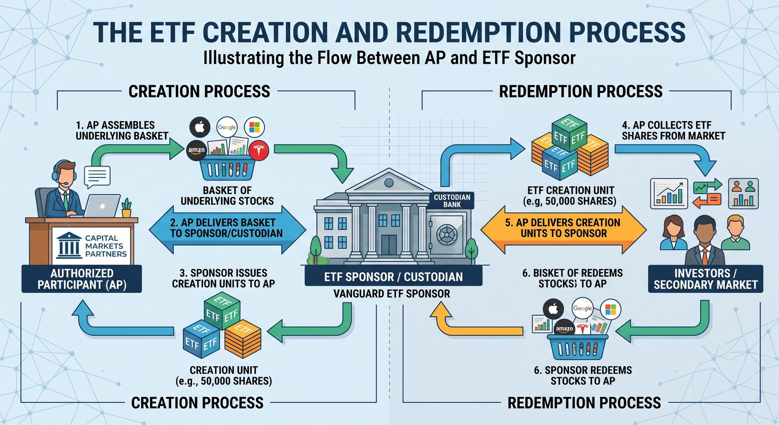
1. The Macroeconomic Mechanics: The Creation and Redemption Process
To understand why an ETF is structurally superior to a Closed-End Fund (CEF) in terms of price tracking, one must delve into the primary market mechanics operated by Authorized Participants (APs). APs are typically large financial institutions, investment banks, or specialized market makers who have entered into a legal agreement with the ETF sponsor (the fund provider, such as Vanguard, BlackRock, or State Street).
The secondary market is where retail investors buy and sell existing ETF shares on the exchange. The primary market, however, is where ETF shares are actually birthed into or extinguished from existence. This process ensures the ETF's market price remains tightly coupled to its Intraday Indicative Value (IIV) or NAV through a continuous arbitrage cycle.
- The Creation Process (Arbitraging a Premium): If surging demand causes an ETF's market price on the exchange to rise above the aggregate value of its underlying assets (trading at a premium), an AP steps in. The AP buys the underlying securities in the open market in the exact proportions of the ETF's index. The AP then delivers this "basket" of securities to the ETF sponsor. In exchange, the sponsor hands the AP a large block of new ETF shares (typically in "Creation Units" of 50,000 to 100,000 shares). The AP then sells these new, cheaper-to-acquire ETF shares on the open market, pocketing the risk-free arbitrage profit. This influx of new supply instantly drives the ETF's secondary market price back down to match its NAV.
- The Redemption Process (Arbitraging a Discount): Conversely, if mass selling pressure pushes the ETF's market price below its NAV (trading at a discount), the AP buys the undervalued ETF shares on the secondary market. The AP then surrenders these ETF shares to the sponsor in exchange for the underlying stock basket. The AP sells the individual stocks on the open market for a profit. This destruction of ETF shares removes supply, pushing the ETF's market price back up to its NAV.
This elegant "in-kind" exchange is the heartbeat of ETF macroeconomic stability. Because securities are physically exchanged rather than sold for cash, the ETF portfolio manager is insulated from capital gains taxes and transaction costs that plague traditional mutual funds when facing heavy redemptions. This gives ETFs a massive structural tax efficiency advantage.
2. Mathematical Foundations & Valuations
While the AP mechanism keeps prices aligned, quantitative evaluation of an ETF requires a firm grasp of several mathematical metrics. The most fundamental is the Net Asset Value (NAV).
The official daily Net Asset Value (NAV) is calculated exactly once per day at market close using the following formula:
NAV = [ ∑i=1n (Pi × Si) + Cash - Liabilities ] / Sharesoutstanding
Where Pi is the closing price of asset i, and Si is the number of shares of asset i held by the fund.
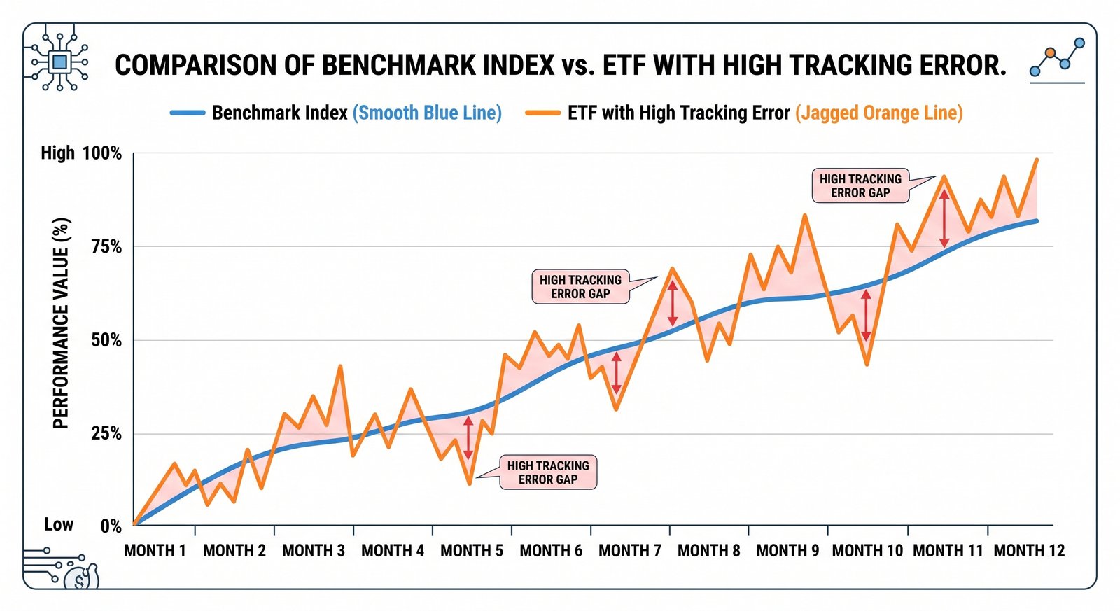
Tracking Error vs. Tracking Difference: For index-tracking ETFs, the goal is not to beat the market, but to replicate it perfectly. Investors use two metrics to judge the quality of this replication. Tracking Difference is simply the annualized return of the ETF minus the annualized return of the benchmark index. It measures exactly how much money you lost to fees and cash drag. Tracking Error, however, is a statistical measure of volatility—specifically, the standard deviation of the difference between the daily returns of the ETF and the daily returns of the index:
TE = √[ ∑i=1N (RETF, i - RIndex, i - μd)2 / (N - 1) ]
Where RETF, i is the ETF return on day i, RIndex, i is the index return, and μd is the mean of the return differences. A low tracking error indicates the fund's manager is tightly hugging the index, regardless of absolute performance.
3. Structural Classifications: Physical vs. Synthetic ETFs
Not all ETFs are built identically. The methodology by which the fund replicates its target benchmark can drastically alter the risk profile presented to the end investor.
- Physical Replication (Full vs. Sampling): This is the most straightforward and common structure. The ETF physically purchases the exact securities contained in the index. In Full Replication, an S&P 500 ETF buys all 500 stocks in their exact market-cap weights. However, for vast, illiquid indices (like a global aggregate bond index with 10,000+ bonds), physical replication uses Optimized Sampling. The manager uses statistical models to buy a representative sample of bonds that mimic the yield, duration, and credit profile of the entire index, reducing transaction costs but introducing a slight degree of tracking error.
- Synthetic Replication (Swap-Based): Popular in Europe and for accessing difficult-to-reach markets (like specific commodity futures or heavily restricted emerging markets), synthetic ETFs do not buy the underlying assets. Instead, the ETF enters into a Total Return Swap agreement with a counterparty (usually a major investment bank). The ETF holds a basket of unrelated collateral (like blue-chip stocks or government bonds), and the counterparty agrees to pay the ETF the exact return of the target index, minus a swap fee. While this achieves incredibly tight tracking error, it introduces Counterparty Risk—if the investment bank defaults during a severe financial crisis, the ETF could suffer losses despite holding collateral.
4. Structured Comparison Table: ETFs vs. Alternative Vehicles
Investors frequently face a choice between deploying capital into Exchange-Traded Funds or traditional Mutual Funds. The table below delineates the precise operational and financial distinctions.
| Feature / Metric | Exchange-Traded Funds (ETFs) | Traditional Open-Ended Mutual Funds |
|---|---|---|
| Trading & Pricing | Trades continuously on exchanges intraday. Priced based on market supply/demand (near NAV). | Trades only once per day. Orders execute at the End-of-Day NAV, regardless of when submitted. |
| Minimum Investment | One share (or fractional share if broker allows). Typically very low barrier to entry. | Often requires a flat monetary minimum (e.g., $1,000, $3,000) for initial entry. |
| Tax Efficiency Mechanics | Highly efficient. AP "in-kind" redemption purges low-cost basis shares without triggering capital gains for remaining shareholders. | Less efficient. Manager must sell stocks for cash to meet redemptions, distributing taxable capital gains to all remaining holders. |
| Execution Control | Supports Limit, Stop-Loss, and Stop-Limit orders, allowing precise entry/exit control. Options trading often available. | Only Market orders executed at the unknown forward EOD price. No advanced order routing available. |
5. Realistic Case Studies
Theoretical knowledge must translate into practical application. The following detailed scenarios illustrate common advanced usage models for ETFs.
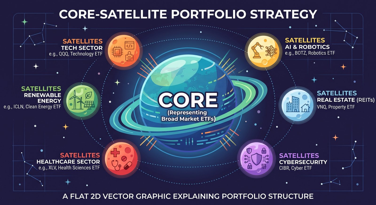
Case Study 1: Sarah’s Core-Satellite Architecture
Sarah, a 35-year-old investor, possesses a $150,000 portfolio and seeks long-term growth with a moderate risk profile. Instead of buying individual stocks, she utilizes a Core-Satellite ETF strategy. She allocates 70% ($105,000) of her capital to her "Core"—an ultra-low-cost Total Global Stock Market ETF (expense ratio 0.08%). This guarantees she captures total global economic growth while mitigating single-country risk. For her 30% "Satellite" allocations ($45,000), she takes active bets on sectors she believes will outperform. She allocates $20,000 to a Semiconductor ETF, $15,000 to an Emerging Markets Dividend ETF, and $10,000 to a long-duration Treasury Bond ETF as a volatility hedge. By utilizing ETFs, Sarah achieves a globally diversified, precisely weighted portfolio with massive liquidity for less than 0.20% average annual fees.
Case Study 2: Volatility Decay in Leveraged ETFs (The Edge Case)
David, a speculative trader, believes the S&P 500 will rise over the next month. He purchases $10,000 of a 3x Daily Leveraged Bull ETF. However, he holds the ETF during a highly volatile, yet ultimately flat, 5-day market period.
- Day 1: Index rises 5%. The 3x ETF rises 15%. David’s balance is $11,500.
- Day 2: Index falls 5%. The 3x ETF falls 15%. Balance becomes $9,775.
- Day 3: Index rises 4%. The 3x ETF rises 12%. Balance becomes $10,948.
- Day 4: Index falls 4%. The 3x ETF falls 12%. Balance becomes $9,634.
Even though the underlying index is virtually flat (down roughly 0.36% geometrically), David's leveraged ETF has lost nearly 3.7% of its value. This phenomenon, known as Volatility Decay or Beta Slippage, mathematically proves that daily reset leveraged ETFs are designed exclusively for intraday tactical trades, not long-term hold strategies. The daily compounding of returns destroys capital in choppy, sideways markets.
6. Advanced Edge-Cases: Contango in Commodity ETFs
When an investor purchases a physical stock ETF, they own fractional shares of businesses. When purchasing a Commodity ETF (like Oil or Natural Gas), the ETF rarely holds physical barrels of oil in a vault. Instead, it holds front-month futures contracts. This introduces the phenomenon of Contango.
Contango occurs when the futures price of a commodity is higher than the current spot price, often due to storage costs and insurance (the Cost of Carry). Because futures contracts expire, the ETF manager must constantly sell expiring contracts and buy the next month's contracts to avoid taking physical delivery. If the market is in contango, the manager is repeatedly "selling low and buying high" during this roll process. Over time, this roll yield is deeply negative, meaning an oil ETF can severely underperform the actual spot price of crude oil over a 12-month period, crushing long-term holders.
7. Actionable Strategy Guide: Building Your ETF Portfolio
Executing a successful ETF strategy requires systematic discipline to avoid execution pitfalls and excessive fees. Follow this step-by-step framework to initiate your positions:
- Step 1: Define Asset Allocation via Risk Capacity. Determine the ratio of Equities to Fixed Income based on your time horizon. A standard baseline is 80/20 (Stocks/Bonds) for an investor 15+ years from retirement, shifting to 60/40 as retirement approaches.
- Step 2: Screen for Total Expense Ratio (TER) and AUM. When comparing similar ETFs (e.g., three different S&P 500 ETFs), filter by TER (aim for under 0.10% for core broad-market funds). Furthermore, ensure the ETF has an AUM of at least $500 million. Low AUM funds risk liquidation, which can trigger an unexpected taxable event.
- Step 3: Evaluate Liquidity via the Bid-Ask Spread. Never assume high AUM equals perfect liquidity. Check the spread (the difference between the highest price a buyer is willing to pay and the lowest price a seller will accept). Narrow spreads (e.g., $0.01) mean minimal friction costs. Wide spreads erode your capital upon entry and exit.
- Step 4: Execute via Limit Orders. ETFs trade intraday, meaning a sudden "Flash Crash" or a momentary lapse in AP arbitrage can cause the market price to detach wildly from NAV. Never use a "Market Order" to buy an ETF. Always use a "Limit Order" set a few cents above the current ask price to protect yourself from algorithmic price spikes.
- Step 5: Avoid the Opening and Closing Bells. Do not trade ETFs in the first 15 minutes of the market open or the last 15 minutes before the close. Early in the day, underlying stocks are undergoing price discovery, causing APs to widen spreads due to uncertainty. Mid-day trading usually offers the tightest spreads and closest alignment to IIV.
8. Frequently Asked Questions (FAQs)
Q: How do Accumulating ETFs handle dividend payments compared to Distributing ETFs?
Distributing ETFs pay out the dividends generated by the underlying stocks directly to the investor's brokerage account as cash, usually quarterly. Accumulating ETFs, more common in European markets, automatically reinvest these dividends back into the fund itself on the ex-dividend date. This increases the fund's NAV without distributing cash, providing massive tax deferral benefits in jurisdictions where dividend payouts trigger immediate taxation.
Q: If an ETF goes bankrupt or shuts down, do I lose all my invested money?
No. If an ETF sponsor decides to liquidate a fund (usually due to lack of investor interest and low AUM), the ETF is legally separate from the sponsor's corporate balance sheet. The underlying assets held in the custodian bank are systematically sold off over a few weeks, and the resulting cash is distributed proportionally to the shareholders based on the final NAV. The primary risk is not total capital loss, but rather receiving a forced cash distribution at an inopportune time, which may trigger unexpected capital gains taxes.
Q: Why should I focus on 'Implied Liquidity' rather than 'Average Daily Trading Volume' (ADTV)?
Many investors mistakenly believe an ETF is illiquid if it only trades 10,000 shares a day. However, an ETF's true liquidity is dictated by the liquidity of its underlying basket of securities, not its ADTV on the secondary market. If a newly launched ETF holds highly liquid mega-cap stocks like Apple and Microsoft, Authorized Participants can easily create millions of new ETF shares instantly. Therefore, its "Implied Liquidity" is immense, and you can place large block trades without moving the market price, despite low historical trading volume.
Q: What are the specific dangers of investing in 'Inverse' or 'Short' ETFs?
Inverse ETFs use complex derivatives (swaps and futures) to deliver the opposite daily return of an index. Like leveraged ETFs, they reset daily. In trending markets, they can work as intended, but in oscillating markets, beta slippage will erode the capital. Furthermore, they carry heavy counterparty risks, higher expense ratios (often 0.90%+), and should solely be utilized by sophisticated traders as short-term tactical hedges, never as buy-and-hold portfolio foundations.
Q: Can I owe taxes on an ETF even if I haven't sold any shares?
Yes, though it is far less common than with mutual funds. If the ETF holds bonds or dividend-yielding stocks and distributes those earnings, you owe taxes on that income for the year it is received. While the ETF creation/redemption process shields investors from most internal capital gains distributions resulting from portfolio rebalancing, a massive rebalance (such as a company being removed from the S&P 500) could theoretically force the ETF to realize capital gains that cannot be fully offset via "in-kind" redemptions, though portfolio managers utilize advanced tax-loss harvesting to prevent passing these onto the shareholder.
See also
- Loading related topics...