Time Value of Money
The Definitive Guide to Compounding, Discounting, and the Temporal Architecture of Capital
The Time Value of Money (TVM) is unequivocally the most fundamental, inescapable mathematical concept in modern finance, economics, and investment theory. At its core, the TVM principle asserts a simple but profound universal truth: a specific, nominal sum of money is worth objectively more today than that exact identical sum will be worth at any point in the future. This structural discrepancy in value is driven by the inherent potential earning capacity of money over time. Provided that capital can be deployed to earn interest, yield dividends, or capture capital gains, any amount of money possessed in the present contains a latent future value that mathematically exceeds its current nominal face value. Consequently, rational economic actors will consistently demand a premium for deferring consumption and parting with their capital, universally preferring to receive a dollar today over receiving a dollar tomorrow.
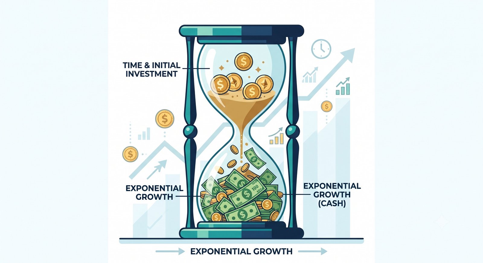
Understanding the mechanics of the Time Value of Money is the absolute prerequisite for making informed, mathematically sound financial decisions. It is the underlying engine that drives everything from everyday personal finance choices—such as calculating the exact amortization schedule of a 30-year residential mortgage or projecting the terminal value of a retirement account—to highly complex corporate finance operations, such as capital budgeting, mergers and acquisitions, discounted cash flow (DCF) corporate valuation, and sovereign bond pricing. Without the framework of TVM, it would be mathematically impossible to compare cash flows that occur at different temporal periods, rendering modern financial analysis, lending, and investment strategy functionally unworkable.
1. The Three Pillars: Why Present Capital Commands a Premium
The economic logic dictating that present capital holds greater utility than future capital is not an arbitrary banking construct. It is firmly grounded in three distinct, inescapable economic realities that affect every market participant globally: Opportunity Cost, Inflationary Erosion, and Counterparty Risk.
- Opportunity Cost (The Engine of Capitalism): This is the loss of potential mathematical gain from other alternatives when one alternative is chosen. If an investor holds $100,000 today, they possess the immediate, unencumbered opportunity to deploy that capital into a risk-free sovereign bond yielding 5%, a broad-market S&P 500 index fund, or a cash-flowing real estate property. If they agree to lend that $100,000 to a friend and wait five years to receive it back without interest, they have suffered a massive opportunity cost representing five years' worth of forfeited, compounded investment returns.
- Inflationary Pressures (The Invisible Tax): In modern, debt-based fiat monetary systems, central banks systematically target positive inflation (typically ~2% annually). Inflation is a persistent, thermodynamic force that gradually and permanently decreases the purchasing power of currency. As the macroeconomic general price level of goods, services, and labor rises, a nominal dollar buys fractionally less over time. Therefore, receiving $10,000 in ten years means receiving capital that fundamentally wields significantly less economic purchasing power than it does at the present moment. Lenders must charge interest simply to tread water against this inflationary drag.
- Counterparty Risk and Uncertainty (The Hazard Premium): The future is inherently opaque and uncertain. A contractual promise to pay a sum of money in the future carries counterparty risk—the statistical probability that the debtor may default, declare insolvency, or simply abscond. Furthermore, systemic macro-risks (wars, pandemics, regulatory shifts) could alter the economic landscape entirely. Because a dollar currently physically in hand carries zero default risk, it logically commands a heavy premium over a speculative, promised future dollar.
2. The Core Variables of TVM Mathematics
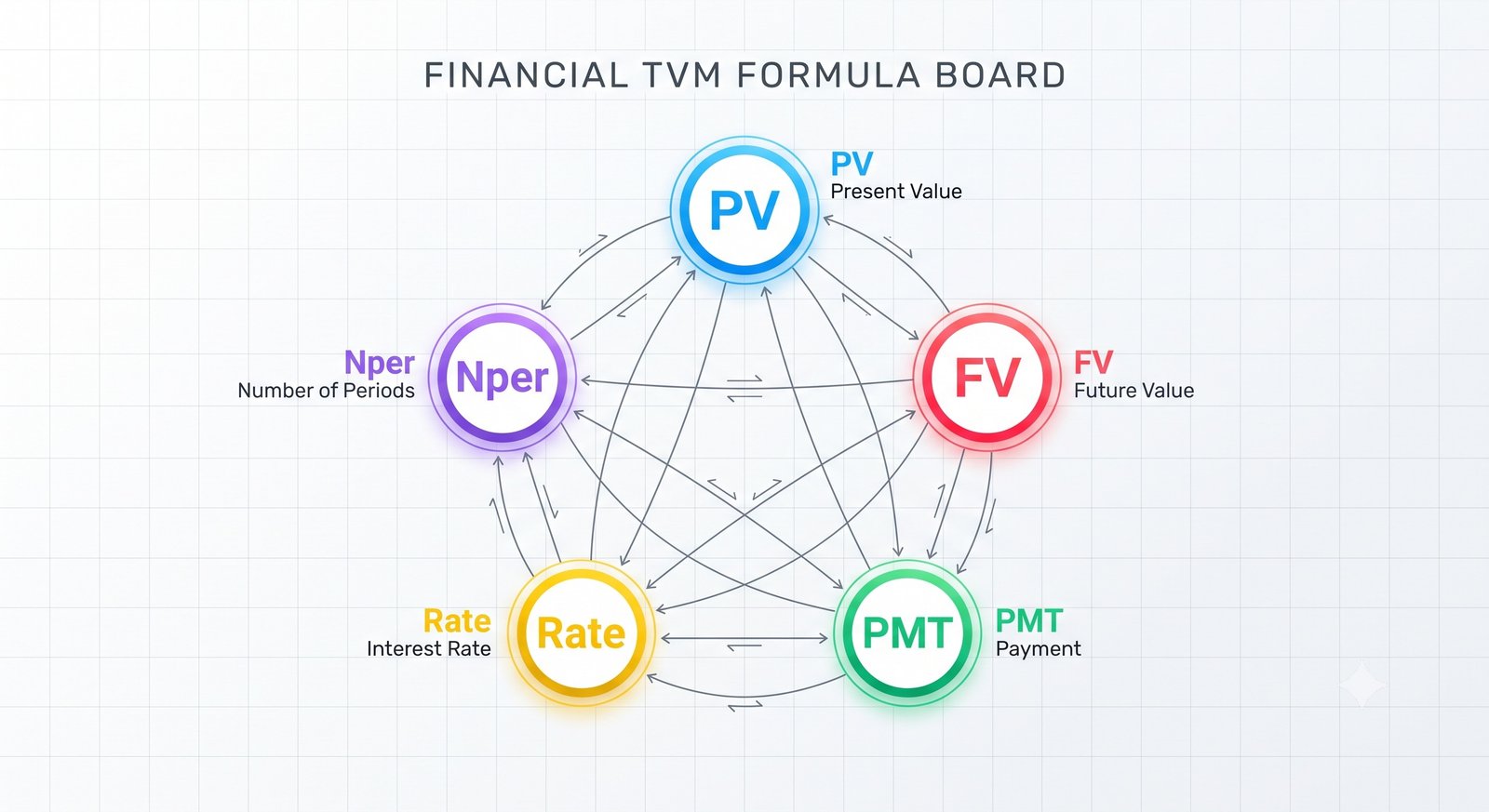
To operationalize the Time Value of Money, financial engineers, actuaries, and software algorithms utilize a standardized set of five variables. These inputs form the unbreakable algebraic foundation of all compounding and discounting formulas globally.
- Present Value (PV): The current, present-day nominal worth of a future sum of money or stream of cash flows, given a specified rate of return. It represents the exact amount of capital that must be invested today to reach a specific target future amount.
- Future Value (FV): The ultimate mathematical value of a current asset at a specified date in the future, based on an assumed, compounded rate of growth. FV answers the fundamental question of how much a present investment will be worth after accumulating and reinvesting interest over a defined horizon.
- Interest Rate / Discount Rate (r or i): The required rate of return or the yield generated over a specific period. This is the mechanism of growth or decay. When projecting forward in time, this is called the compounding rate or interest rate. When calculating backward from the future to determine current value, it is known as the discount rate.
- Number of Periods (n or t): The total temporal length over which interest is applied or cash flows occur. This is typically measured in years, but must be mathematically adjusted for months, quarters, or days depending on the specific compounding frequency of the financial instrument.
- Payment (PMT): A series of equal, periodic cash flows (an annuity). This variable is strictly utilized when money is systematically added to or subtracted from an account on a regular, recurring schedule, such as monthly mortgage payments, bi-weekly 401(k) paycheck deductions, or annual corporate dividend distributions.
3. The Mechanics of Compounding and Discounting
The mathematics of TVM involve two primary, opposing operational directions: Compounding (moving forward in time) and Discounting (moving backward in time).
Compounding (Calculating Future Value)
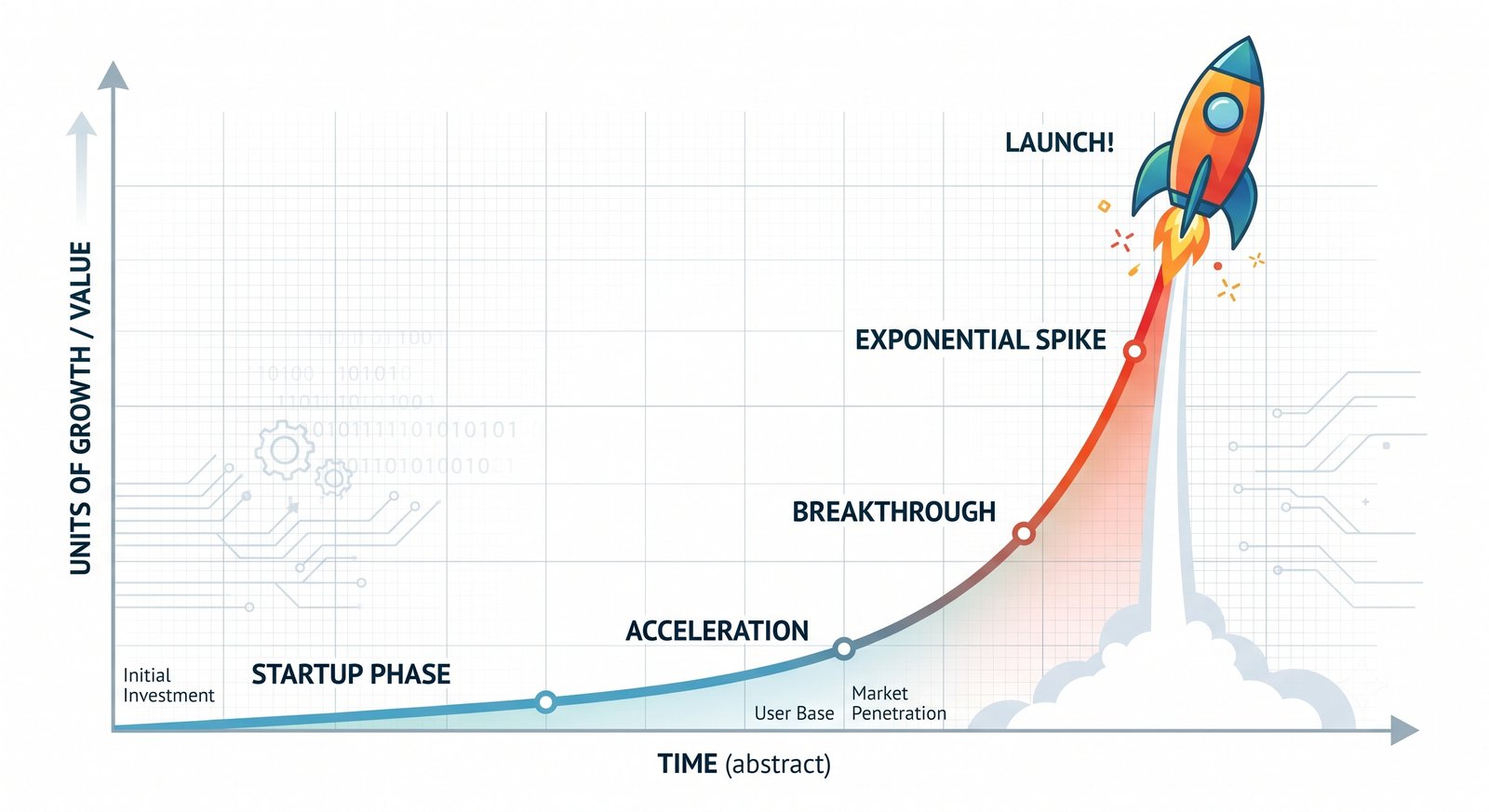
Compounding is the process of moving from Present Value to Future Value. It assumes that any interest earned in a given period is not consumed, but is instead forcefully reinvested to earn additional interest in all subsequent periods, leading to geometric, exponential growth.
Future Value Formula:
FV = PV × (1 + r)^n
For example, if a retail investor deploys a lump sum of $50,000 (PV) into an S&P 500 index fund generating an annualized nominal return of 8% (r = 0.08) and leaves it untouched for 30 years (n = 30), the future value calculation would be $50,000 × (1 + 0.08)^30. The resulting Future Value equates to a staggering $503,132.84. The initial $50,000 capital generated over $450,000 in pure, compound interest.
Discounting (Calculating Present Value)
Discounting is the exact reverse mechanism. It determines the present-day, nominal equivalent of a cash flow expected to arrive in the future, actively adjusting for the opportunity cost of capital (the discount rate). Discounting answers the critical institutional question: "How much money would I need to invest today to guarantee a specific sum in the future, or what is the maximum I should pay for this future asset today?"
Present Value Formula:
PV = FV / (1 + r)^n
If an investor is offered a contract that promises to pay them exactly $1,000,000 in exactly 10 years, and their required rate of return (based on alternative investments available to them in the market) is 7%, the present value equation is $1,000,000 / (1 + 0.07)^10. This equates to a present value of $508,349.29. Consequently, if the investor can purchase this contract today for $400,000, it represents a massive mathematical bargain. If the seller demands $600,000, the investor must decline, as they could generate a better return elsewhere.
4. The Mathematical Impact of Compounding Frequency
A critical, often misunderstood nuance in TVM calculations is the frequency of compounding. Interest is not exclusively calculated and applied on an annual basis; depending on the institutional contract, it can be compounded semi-annually, quarterly, monthly, daily, or even continuously. The higher the compounding frequency, the greater the exponential growth of the asset (or the debt), because interest begins generating its own interest sooner in the temporal cycle.
To account for multiple compounding periods within a single calendar year, the standard TVM formulas must be modified. The annual stated interest rate (r) must be divided by the number of compounding periods per year (m), and the total number of years (n) must be multiplied by that exact same frequency metric to derive the total number of periods.
Adjusted Future Value Formula (Multiple Compounding Periods):
FV = PV × [ 1 + (r / m) ]^(n × m)
| Compounding Frequency | Formula Divisor (m) | Terminal Value of $10,000 at 8% over 20 Years |
|---|---|---|
| Annual (Once per year) | m = 1 | $46,609.57 |
| Quarterly (4 times per year) | m = 4 | $48,754.39 |
| Monthly (12 times per year) | m = 12 | $49,268.03 |
| Daily (365 times per year) | m = 365 | $49,522.65 |
In retail consumer banking, credit card companies and mortgage lenders typically compound interest on a daily or monthly basis. This mathematically accelerates the accumulation of debt for the borrower, resulting in an Effective Annual Rate (EAR) that is significantly higher than the prominently advertised Annual Percentage Rate (APR), maximizing yield for the financial institution.
5. Empirical Case Studies in Time Value Execution
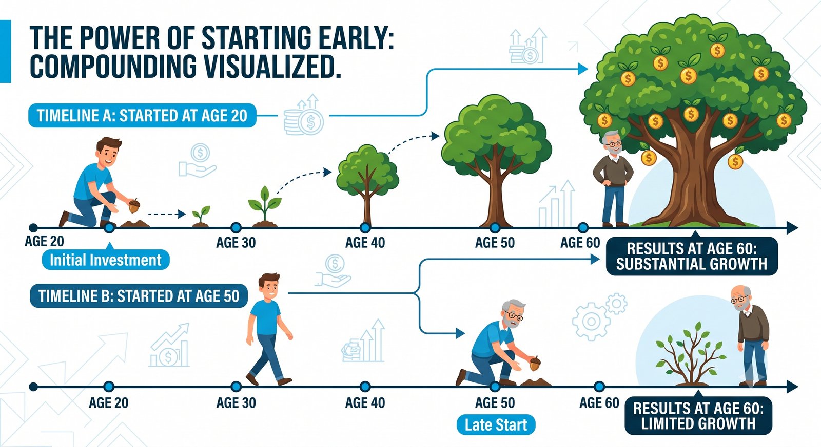
To fully comprehend the unforgiving mechanics of TVM, we must examine its application in specific, real-world financial scenarios.
Case Study 1: The Cost of Delay (Retirement Annuities)
Scenario: Two investors, Alice and Bob, both intend to retire at age 65. Alice begins investing $500 per month (PMT) into an S&P 500 index fund at age 25, stopping completely at age 35 (she invests for only 10 years, contributing a total out-of-pocket principal of $60,000). Bob waits until he is 35 to start, but then aggressively invests $500 per month every single month until he reaches 65 (investing for 30 years, contributing a total out-of-pocket principal of $180,000). Both achieve a nominal annualized return of 8%.
The Mechanics: Utilizing the Future Value of an Annuity formula combined with standard compounding, we evaluate the terminal balances at age 65.
Alice's 10 years of payments grow to $91,473 by age 35. That lump sum then sits untouched, compounding at 8% for 30 more years. Her final balance at age 65 is roughly $920,000.
Bob's 30 years of continuous $500 monthly payments compound directly. His final balance at age 65 is roughly $745,000.
Result: Despite Bob investing three times more physical capital out of his own pocket ($180,000 vs $60,000), Alice retires significantly wealthier. This is the absolute power of the 'n' variable (Time) in the TVM equation. By starting early, Alice allowed compound interest to do the heavy lifting, proving that capital deployed early is mathematically superior to heavy capital deployed late.
Case Study 2: Corporate Valuation (Discounted Cash Flows)
Scenario: A private equity firm is evaluating the purchase of "TechCorp," a mature software company. TechCorp reliably generates $10 Million in Free Cash Flow (FCF) every year. The private equity firm intends to hold the company for exactly 5 years and then sell it. Based on the firm's strict risk profile, their required rate of return (Discount Rate / WACC) is 12%.
The Mechanics: The firm cannot simply multiply $10M by 5 years and value the cash flows at $50 Million. The $10M received in Year 5 is worth drastically less than the $10M received in Year 1. The firm must discount each year's cash flow individually using the PV formula: PV = $10M / (1 + 0.12)^n.
Year 1 PV: $8.93 Million
Year 2 PV: $7.97 Million
Year 3 PV: $7.12 Million
Year 4 PV: $6.36 Million
Year 5 PV: $5.67 Million
Result: The sum of the present value of all 5 years of cash flow is $36.05 Million. If the private equity firm pays $50 Million for those cash flows, they will fail to achieve their 12% target return. TVM mechanics dictate the absolute ceiling of the acquisition price.
6. Actionable Strategy Guide: Deploying TVM in Daily Life
While the mathematics of TVM can be complex, its application in personal financial architecture is highly practical. Utilize the following strategic blueprint to leverage TVM in your favor, transforming time into your primary wealth-generating asset.
- Step 1: Front-Load Investment Capital (Front-Loading). Because the 'n' (time) variable is an exponent, money invested in your 20s and 30s is exponentially more valuable than money invested in your 50s. If you receive a windfall (bonus, tax refund, inheritance), immediately deploy it into growth assets. Delaying deployment by even two years permanently sacrifices the backend compounding tail.
- Step 2: Automate High-Frequency Annuities (SIPs). Do not attempt to "time the market" with annual lump sums. Establish a Systematic Investment Plan (SIP) that auto-deducts capital from your checking account bi-weekly or monthly. This increases the compounding frequency and captures the average market return over time, mathematically ensuring steady future value growth.
- Step 3: Analyze the "Opportunity Cost" of Major Purchases. Before executing a large discretionary purchase (e.g., a $40,000 luxury vehicle), use a TVM calculator to evaluate the future value of that capital. If that $40,000 were instead invested at 7% for 20 years, its Future Value is over $150,000. Frame the purchase decision not as "Does this car cost $40k today?" but rather, "Is this car worth sacrificing $150k in retirement?"
- Step 4: Audit Debt Compounding Frequencies. Understand that banks use TVM against you when lending money. If you hold credit card debt compounding daily at 24% APR, you are bleeding capital geometrically. Prioritize the eradication of high-interest, high-frequency compounding debt above all other financial goals, as it actively destroys your future value.
- Step 5: Demand a Premium for Deferred Compensation. If an employer, business partner, or settlement offers you a payout structured over multiple years rather than an immediate lump sum, you must mathematically discount the future payments. The total sum of the deferred payments must significantly exceed the lump sum offer to compensate you for inflation, counterparty risk, and the loss of investment yield.
7. Frequently Asked Questions (FAQ)
Q: Is TVM only relevant for rich investors and massive corporations?
Absolutely not. TVM governs the financial reality of every single participant in the economy. Every time you take out a car loan, swipe a credit card, deposit $100 into a savings account, or choose to rent instead of buy, you are actively executing a TVM equation. Wealthy individuals simply understand the mathematics and structure their lives so that the exponent (interest) compounds in their favor, while the financially illiterate allow the exponent to compound against them via debt.
Q: Why does the bank charge me more total interest on a 30-year mortgage than a 15-year mortgage if the interest rate is the same?
This is the purest demonstration of TVM. Because you are holding the bank's capital for twice as long (30 years vs 15 years), the bank suffers twice the opportunity cost and twice the inflationary risk. To compensate, the loan amortization schedule is mathematically structured so that the compounding interest accumulates over 360 monthly periods instead of 180. The time variable (n) dictates the total cost of the capital.
Q: How do I choose the correct 'Discount Rate' when calculating Present Value?
The discount rate is entirely subjective and depends on the specific investor's opportunity cost and risk tolerance. A common baseline is the "Risk-Free Rate," typically represented by the yield on a 10-Year US Treasury Bond (e.g., 4%). If you are evaluating a highly risky private business venture, you might demand a much higher discount rate (e.g., 15%) to compensate for the probability of default. In personal finance, individuals often use an expected stock market return (7% to 9%) as their baseline discount rate when evaluating choices.
Q: If inflation is currently 5%, but my bank account pays 2%, what is happening to my TVM?
You are experiencing a Negative Real Return. While your nominal Future Value is mathematically increasing (your bank balance goes up), the actual economic purchasing power of that money is decaying by roughly 3% per year. In real terms, the TVM equation is functioning in reverse—your present capital is buying fewer goods in the future. This forces rational actors to move capital out of cash and into higher-yielding, riskier assets to outpace the inflation metric.
Q: What is the Rule of 72, and how does it relate to TVM?
The Rule of 72 is a highly accurate mental heuristic (shortcut) used to estimate how long it will take an investment to double in value via compound interest, without requiring a complex financial calculator. You simply divide the number 72 by the annual interest rate. For example, if you invest $10,000 at a 9% annual return, it will take exactly 8 years (72 / 9 = 8) for that capital to reach $20,000. It is a quick-math manifestation of the Future Value formula.
See also
- Loading related topics...